Kernel Development
NPU HW Overview
Torq NPU consists of a number of processing units called Slice. The slices are independent but share a common local RAM (LRAM). Slices cannot access DRAM directly, all data, constants, programs and results must be located in LRAM.
Each slice contains an ALU, and an activation unit (Act): these are SIMD units capable of vector processing. In addition the slice contains a few internal memories that can be used as caches or transfer buffers. ALU, Act and the internal memories are connected by programmable transfer agents called NDL.
All these components operate in parallel to perfom a computation.
Programming a Slice
Performing a computation with a Slice requires configuring the ALU, the Act and all the NDLs. A configuration that performs a specific computation is called a kernel.
Developing a kernel that runs on a Torq Slice using low-level HW APIs to program each unit directly is a complicated activity. Complications are due to multiple reasons:
Programming a vectorized architecture is intrinsically harder then normal SISD programming and requires correct data organization and processing to exploit parallelism
Idiosyncrasies and peculiarities in the HW (HW is optimized for efficiency not for easiness of programming)
Each NDL must be programmed with the counts, strides and offset of the data to be trasferred. Working with mutiple groups of counts and strides is unnatural and error-prone.
Multiple parallel but interdependent data flows are difficult to grasp by SW people
How can we write efficient kernels without getting lost in this complexity?
Carefully design the data organization (e.g.: put data that can be processed together close to each other, provide adequate alignement and padding if needed). Design the processing to reduce the number of times the same data is copied in/out from local memory.
Encapsulate the specific HW behaviour inside higher-level operations This allows us to provide a logical “instruction set” for the NPW which abstract the HW details (eg. multiplyAccumulate instruction)
Organize the data in multi-dimensional tensors with a shape and element type. Let the internal implementation take care of the corresponding sizes, strides and offset (same idea as numpy).
In our Torq Slice the data flows (represented by the NDLs) are running in parallel but they are not completely independent, actually they must be exactly syncronized in order to get the correct results. Even if we have about 10 of these data flows, they represent one single computation. Let’s express the overall computation once and derive all the data flows from there.
EasyKernel is a library designed to help kernel writers with points 2. 3. and 4. It allows to generate the low-level settings and NDLs configuration from a more natural higher-level description.
Even with this support, kernel writing is definitely not easy: organizing data in a proper way and using the right instructions to parallelize processing as much as possible remains an important design challange.
EasyKernel
EasyKernel provides a C++ API that allows to express a kernel using high-level constructs. It provides a simplified logical view of a Torq Slice that abstracts many of the details and complexities of the underlying HW implementation.
The picture here below shows a logical diagram of a Slice as presented by the EasyKernel library:
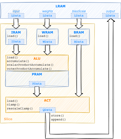
The slice contains:
2 computational units (ALU and Act)
4 internal memories: IRAM, WRAM, BRAM used as cache or temporary buffers to contain respectively input, weights and (bias,scale) values. PRAM is used by ALU as a working memory to contain partial results.
Each unit provides its own instruction set. PRAM has no instructions since it is controlled directly by the ALU. The NDL data-transfer engines are not represented in this view since their configuration is derived implictly from the instructions of the other components.
LData structures are used to repesent n-dimensional tensors in LRAM.
Each tensor has a data type and n dimensions, each with its own element count and stride.
Representing the strides explicitly provides a natural way to represent data which is not
contiguous in memory. The concept is very similar to that of a MemRef in MLIR.
In the same way we use IData, WData, BData, PData structures
to represent tensors in IRAM, WRAM, BRAM and PRAM respectively.
These data structures all work essentially the same, the main difference is the physical location
of the data they represent.
EasyKernel allows to express a kernel as a sequential program using these instructions and data types. It’s important to keep in mind that despite this illusion of sequentiality, during execution all the unit in a Slice will actually operate in parallel.
Tutorial
The best way to explain how to write a kernel is probably with an example. In this section we will see how to write a simple kernel that performs elementwise multiplication of two input tensors. We will start with some strict assumptions on the format of the input data and then see how to extend the kernel to be completely generic while still being as efficient as possible.
Vector Multiplication (basic)
In this example we want to write a kernel to perform element-wise multiplication of two vectors.
Required kernel behaviour: receive in input two tensors of rank 1 and generate in output a tensor containing the rescaled elementwise products of the inputs, clamped to a specified min and max values. Rescale is specified with a bias and scale value (the same for all the elements). Each output value must be computed as:
out[i] = clamp((input1[i] * input2[i] + bias) * scale, min, max)
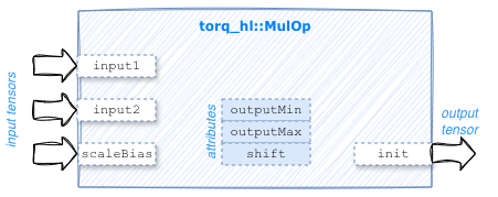
The higher level compiler passes will create a torq_hl::MulOp object representing the operation:
Our job as kernel writers is to specify how this operation will be executed by the Torq slice. The easiest way to start writing a kernel is to use the Slice as a scalar (SISD) processor on input tensors with a known shape.
The first thing to do when developing a kernel is to define the data tensors in LRAM on which the
kernel will operate.
Normally the data shape, layout, and type of these tensors cannot be decided by the kernel but come from
higher-level compiler passes via MemRef structures.
Each MemRef is associated to an operand of an MLIR operation and can be accessed with the name of the operand.
Conveniently LData objects can be created directly from MLIR operands.
We also create a Slice object that will allow us to express the
computation using high-level instruction and translate them to the corresponding HW and NDL configuration.
Slice slice;
LData input1(op.getInput1());
LData input2(op.getInput2());
LData biasScale(op.getScaleBias());
LData output(op.getInit());
In addition to operands, MLIR operators also have attributes that can also be accessed by name, so we can get the min and max output values, and the shift needed for the rescale:
const int outMin = op.getOutputMin();
const int outMax = op.getOutputMax();
const int shift = op.getShift();
It’s also always a good idea to verify that the tensors are as expected:
// Verify inputs are 1D and same length
assert(input1.shape().size() == 1 && input2.shape().size() == 1);
assert(input1.dim(0) == input2.dim(0));
Now that the data definition is completed we can start to define the algorithm to perform the processing. The Torq Slice is not able to use data from LRAM directly, we have first to bring them to one of the internal memories (IRAM, WRAM or BRAM). In our case the biasScale tensor is very small (it contains only one [bias, scale] pair) so we can simply bring it to internal memory once at the beginning and leave it there.
BData bdata = slice.bram.load(biasScale);
Now we can start specifying the processing. The idea is to perform the same computation for all the elements in the input tensors, one value at a time. We need a for loop:
For(auto i = slice.iterate(input1.dim(0))) {
    // Body of the processing to be added here
}
Important
The uppercase F in the above code is not a typo. And this is not a real C++ loop. This is just a syntactic representation of a loop that will be executed by the Slice.
We can see iterate(N) as a method that creates an iterator representing a loop that will be repeated N times.
Here N is input1.dim(0) that is the number of elements in the first (and only) dimension in input1.
Each iterator internally contains an iteration variable that represents a runtime
index incrementing from 0 to N-1. We can use these iteration variables as indexes to extract parts
of the data tensors.
Now let’s fill the body of our loop.
We can access values in the LData tensors by indexing them as we would do with standard arrays and
multiply each element of the first input by the corresponding element of the second input.
The Alu class contains the full list of instruction it supports.
Two of them could be used here: scalarProductAccumulate or elementwiseProductAccumulate.
In the former the second operand must be a scalar, while in the latter it can be a scalar or a vector.
We use elementwiseProductAccumulate since it will be compatible with the improved versions
of this kernel what we will develop below.
The first argument of this instruction is of type IData
while the second one is of type WData: this means that we have to bring the corresponding
operands in IRAM and WRAM respectively. This can be done using the load() instruction.
At each iteration we will load one element of the first vector in IRAM and one element of the
second vector in WRAM, then multiply them.
We specify which element to load by indexing the corresponding input with the iteration variable defined
in the For loop:
IData data1 = slice.iram.load(input1[i]);
WData data2 = slice.wram.load(input2[i]);
PData pdata = slice.alu.elementwiseProductAccumulate(data1, data2);
Since both arguments contains one single value, the resulting pdata will also contain one single value.
We can rescale and clamp this value using the activation unit (rescaleClamp instruction in the Act class)
and store the result in the output tensor.
This completes the definition of the kernel, here the complete code:
// Verify inputs are 1D and same length
assert(input1.shape().size() == 1 && input2.shape().size() == 1);
assert(input1.dim(0) == input2.dim(0));

BData bdata = slice.bram.load(biasScale);
For(auto i = slice.iterate(input1.dim(0))) {
    IData data1 = slice.iram.load(input1[i]);
    WData data2 = slice.wram.load(input2[i]);
    PData pdata = slice.alu.elementwiseProductAccumulate(data1, data2);
    QData res = slice.act.rescaleClamp(pdata, bdata, shift, 0, outMin, outMax);
    slice.store(output[i], res);
}
We can now ask the Slice object to provide the corresponding HW settings and NDLs configuration using
the getCfgAttr() and getNdls() methods.
Using the Slice as a scalar processor is not very different from writing the same operation in C for a standard CPU. Of course this is not using the full computational power of the Slice, we will see how to improve this in the next version of this kernel.
Tip
Writing a basic version of a kernel operating one element at a time can often be a good way to start designing a kernel, since this doesn’t require any specific data organization and can provide a reference against which to benchmark more optimized implementations.
Vector Multiplication (vectorized)
In this example we examine how to improve the previous version of the kernel to take advantage of the vector processing features of the ALU and Act units.
The idea is similar to what we have seen before, but instead if operating on one value at a time we operate on vector of values at a time. Of course this is only possible if the data in the input and output vectors are contiguous, that is if they are dense tensors, so we have to check that this is indeed the case:
// Verify inputs and output and dense
assert(input1.denseDims() > 0 && input2.denseDims() > 0 && output.denseDims() > 0);
In order to be able to process multiple input values at a time we need two things:
determine how many values can be processed in parallel, that it the size of the input vectors
split the input tensors in vectors of the given size
The vector size depends on the data type and the HW unit that we want to use. Since the ALU can support bigger vector sizes than the Act, but we want to use the same vecors for both, we ask Act to provide its maximum vector width for the input and weight types we want to use:
int vectorSize = slice.act.width(input1.elementType(), input2.elementType());
Now we can partition each input vector in chunks (vectors) each containing vectorSize elements. For the moment let’s also vectorize the output tensor, we will see soon why this is not a good idea.
input1.vectorize(vectorSize);
input2.vectorize(vectorSize);
output.vectorize(vectorSize);  // /!\ Vectorizing output is deprecated
What happens here is that the input and output tensors are reshaped from a vector of shape [N]
to a 2D tensor of shape [N / vectorSize, vectorSize].
The rest of the code will remain unchanged:
BData bdata = slice.bram.load(biasScale);
For(auto i = slice.iterate(input1.dim(0))) {  // iterate over all the data vectors
    IData data1 = slice.iram.load(input1[i]);
    WData data2 = slice.wram.load(input2[i]);
    PData pdata = slice.alu.elementwiseProductAccumulate(data1, data2);
    QData res = slice.act.rescaleClamp(pdata, bdata, shift, 0, outMin, outMax);
    slice.store(output[i], res);
}
So while in the previous example input1[i] was referring to a single element, the same syntax
applied to the 2D tensor above will actually refer to a vector of vectorSize elements.
The intersting thing is that since the instructions we used inside the For loop in the previous
example (load, store, elementwiseProductAccumulate, rescaleClamp) are all able to work on vectors
of data, there is no need to apply any change to the loop itself, instead of iterating on all the
data elements it will now iterate on all the data vectors. By adding the few lines above we
have transformed the tensor multiplication kernel into one using vector operations.
This new kernel is typically about 10 times faster than the original one (the exact number
depending on the data types).
We still have an important point to address: what happens if the vector size N is not a multiple of
vectorSize?
When we vectorize() a tensor, its size will become a multiple of the specified vectorSize.
For the input tensors this is not a real issue, the last vector will go beyond the end of the
data, so the final elements will contain junk data. Processing junk data is completely legal
as long as they are not used as to compute the valid part of the result.
For the output tensor the situation is different: it is not allowed to write beyond the end of the
tensor, since this will corrupt whatever information is there.
This is checked by the compiler so if we try to use our vecotorized kernel on an data vector that
is not multiple of vectorSize we will get a compile-time error.
One possible solution is for the kernel to explicitly request its output to be padded.
In this way the junk result values from the last vector will safely end up in a padding area that is not used
for anything else. While this approach works, the addition of this additional padding area to the output
tensor can in some cases bbecome quite annoying, for example when working on subviews of existing tensors.
A better solution is to avoid going beyond the end of the output tensor in the first place. Luckily this can be achieved with a simple change to our kernel.
Instead of writing the result to the output tensor using the store() instruction,
we can use the append() instruction.
Append will append the given result to what has already be written in the indicated output (sub)tensor.
So slice.append(output, res) will append res to the results already written in the
output tensor in previous iterations. In the same way slice.append(output[i], res) will append res
to the results already written in the output[i] subtensor in previous iterations.
What makes append() so useful is that it never overflows the size of the output (sub)tensor it is writing.
For example if we try to append two 16-bytes results to a tensor of size 20, the first append will write the
entire 16 bytes, while the second append will just write the initial 4 bytes and discard the remaining 12.
In order for this to work we just have to make sure not to modify the size of the output tensor,
this is why we shall never apply vectorize() to an output tensor.
Here is the final code of our vectorized kernel working on any dense 1D input of any size without any padding:
// Verify inputs are 1D and same length
assert(input1.shape().size() == 1 && input2.shape().size() == 1);
assert(input1.dim(0) == input2.dim(0));

// Verify inputs and output are dense
assert(input1.denseDims() > 0 && input2.denseDims() > 0 && output.denseDims() > 0);

// Vectorize inputs
int vectorSize = slice.act.width(input1.elementType(), input2.elementType());
input1.vectorize(vectorSize);
input2.vectorize(vectorSize);

BData bdata = slice.bram.load(biasScale);
For(auto i = slice.iterate(input1.dim(0))) {
    IData data1 = slice.iram.load(input1[i]);
    WData data2 = slice.wram.load(input2[i]);
    PData pdata = slice.alu.elementwiseProductAccumulate(data1, data2);
    QData res = slice.act.rescaleClamp(pdata, bdata, shift, 0, outMin, outMax);
    slice.append(output, res);
}
Important
Use vectorize() to reorganize the innermost dimension of input tensors for vector processing.
Never vectorize output tensors. Use the append() instruction to write vector results to output
without overflow.
For more info about vectorization please refer to the Vectorization section in the Easykernel reference.
Tensor multiplication (vectorized)
In practice the input and output tensors of an elementwise mul operation are not required to be
vectors with one dimension, they can have any number of dimensions as long as the tensors have the same shape.
Let’s see how to extend our kernel to handle this.
For the case of rank-2 tensors, the change would be trivial, instead of one For loop,
we would now need two nested loops:
For(auto i = slice.iterate(input1.dim(0))) {
    For(auto j = slice.iterate(input1.dim(1))) {
        IData data1 = slice.iram.load(input1[i][j]);
        WData data2 = slice.wram.load(input2[i][j]);
        PData pdata = slice.alu.elementwiseProductAccumulate(data1, data2);
        QData res = slice.act.rescaleClamp(pdata, bdata, shift, 0, outMin, outMax);
        slice.append(output, res);
    }
}
For the case of rank-3 tensors, the change would be trivial as well, we simply need 3 loops. The problem is that we don’t know a priori how many dimensions the tensors can have, and writing an explicit implementaton for each possible rank is tedious end error prone.
For these situations it is very convenient to use an extension provided by the iterate() method.
Instead of passing a single iteration couter, it’s also possible to pass a vector of counters.
In this case we will get as return value not a single iterator but a vector of iterators,
for simplicity we call this a multi-iterator.
A single For loop on a multi-iterator with M elements will be expanded to M loops,
each with its own counter. A multi-iterator will contain a multi-iteration-variable
that can be used to index multiple dimension of a tensor at once.
As concrete example consider the following code:
For(auto m = slice.iterate({4, 7})) {
    IData data = slice.iram.load(input[m]);
    // ...
}
It is equivalent to the code here below:
For(auto i = slice.iterate(4)) {
    For(auto j = slice.iterate(7)) {
        IData data = slice.iram.load(input[i][j]);
        // ...
    }
}
The number of elements in the vector of counters passed to iterate() can be arbitary, including 0 elements.
In this case the multi-iterator will be equivalent to no loops at all:
For(auto m = slice.iterate({})) {
    IData data = slice.iram.load(input[m]);
    // ...
}
is equivalent to:
IData data = slice.iram.load(input);
// ...
With this functionality it’s trivial to write a version of the mul kernel that works with any input rank,
all we have to do is to replace the single iterator with a multi-iterator iterating on all the tensor
dimensions except the last one. Remember that the last dimension is the one representing the elements
of data vectors that we wqnt to process. If we iterated also on this dimension we would be back
processing one element at a time.
We can express “all the input dimensions except the last one” as
input1.dim(0, input1.shape().size() - 1) or equivalently as input1.dim(0, -1) (negative
indexes count from the end as in numpy).
To resume, the change to support tensors of arbitrary rank consist of replacing the line:
For(auto i = slice.iterate(input1.dim(0))) {
with:
For(auto i = slice.iterate(input1.dims(0, -1))) {
Here the full code:
// Verify that inputs have the same rank and the same count in each dimension
assert(input1.dims() == input2.dims());

// Verify inputs and output inner dimensions are dense
assert(input1.denseDims() > 0 && input2.denseDims() > 0 && output.denseDims() > 0);

// Vectorize inputs
int vectorSize = slice.act.width(input1.elementType(), input2.elementType());
input1.vectorize(vectorSize);
input2.vectorize(vectorSize);

BData bdata = slice.bram.load(biasScale);
For(auto i = slice.iterate(input1.dims(0, -1))) {
    IData data1 = slice.iram.load(input1[i]);
    WData data2 = slice.wram.load(input2[i]);
    PData pdata = slice.alu.elementwiseProductAccumulate(data1, data2);
    QData res = slice.act.rescaleClamp(pdata, bdata, shift, 0, outMin, outMax);
    slice.append(output, res);
}
Note that we didn’t change the assert on the dimensions being dense. This is because we actually
need only the innermost dimension to be dense, so that we can vectorize it.
We don’t care about upper dimensions being dense or not since the multi-iterator will automatically
get the correct count and stride for each dimension from the LData structure.
Tip
multi-iterators and the corresponding multi-indexes allow to handle in a generic way
computations involving a variable number of dimensions. A multi-iterator can be created by
calling the Slice iterate() method with a vector of counters.
Important
LData::dim(int index) returns the number of elements in the specified dimension.
LData::dims(int begin, int end) returns a vector with the number of elements in the dimensions
from begin (included) to end (excluded). Negative indexes are interpreted from the end as in numpy.
Tensor multiplication (optimized)
There is still a case where the n-dimensional mul kernel we’ve seen in the previous section is sub-optimal. Imagine that both inputs and output are dense tensors with many small dimensions, for example [5, 3, 3, 2]. Our kernel will vectorize the innermost dimension, giving 1 single vector of 2 elements. Then it will iterate 5 * 3 * 3 times to process all the elements. But since the tensors are dense we could have used bigger vectors than with just 2 elements, this would have required much less iterations.
The idea to improve performnce in these cases is to fuse together as many inner dimensions as
possible. Of course we can only fuse dimensions that are dense. Dimensions that have “holes” in the
data, that is that use non-natural stride cannot be fused. Furthermore since an elementwise
kernel requires the input and output tensors to have the same rank, we can only fuse two nearby
inner dimensions if they are dense in both inputs and ouput tensors.
Note again that we are only talking about inner dimensions.
After we find a non-dense dim we don’t care if outer dimensions are dense or not, we will not be able
to fuse them anyway.
The LData class provides several tensor-editing method, we have already used vectorize() we will
now use fuse():
// Count how many dense inner dimensions we have in input and output
int inDenseDims = std::min(input1.denseDims(), input1.denseDims());
int outDenseDims = output.denseDims();

// Fuse dense dimensions in all the tensors
int denseDims = std::min(inDenseDims, outDenseDims);
input1.fuse(denseDims);
input2.fuse(denseDims);
output.fuse(denseDims);
After this fusion, all tensors will have one inner dense dimension (as big as possible) and possibly additional outer dimensions as needed. The rest of the code will remain unchanged. Vectorization will now operate on a larger inner dimension, and so will be able to make full use of the max vector size supported by the Slice. The above code is completely generic and will work also in the case where there is no dense dimension at all.
Another feature that is quite useful in elementwise operations like mul is broadcasting.
Broadcasting is a mechanism that allows to perform elementwise operations on arrays of different
shapes and sizes without making unnecessary copies of data. For example if this operator
receives input1 having shape [2, 5, 7] and input2 having shape [1, 1, 1] to generate an output
of shape [2, 5, 7], we would like all elements in tensor1 to be multiplied by the single element in input2.
This can be implemented using tensor editing, using the broadcastAs() method.
It will adapt the number of elements in an input tensor to make it equal to the number of
elements in a given output tensor, while at the same time setting the strides correctly
so that the elements in the broadcasted dimensions will be repeated as many times as needed
without being physically duplicated. This is normally done right at the beginning of the kernel
before vectorization is applied:
// Apply implicit broadcasting
input1.broadcastAs(output);
input2.broadcastAs(output);
With the above code we can remove the requirement that the two inputs must have the same rank. Of course the input and output tensors must be compatible for broadcast, otherwise we will get a compile error.
Here is the final version of our mul kernel (we have combined fusion and vectorization). This doesn’t look very different from the basic version we have shown at the beginning, but it can support tensors of any element type, any rank, dense or not dense, broadcasting without data copy, does not require any special memory padding and is optimally efficient.
// Apply implicit broadcasting
input1.broadcastAs(output);
input2.broadcastAs(output);

// Count how many dense inner dimensions we have in input and output
int inDenseDims = std::min(input1.denseDims(), input1.denseDims());
int outDenseDims = output.denseDims();
int denseDims = std::min(inDenseDims, outDenseDims);

// Fuse and vectorize inputs
int vectorSize = slice.act.width(input1.elementType(), input2.elementType());
input1.fuse(denseDims).vectorize(vectorSize);
input2.fuse(denseDims).vectorize(vectorSize);
output.fuse(denseDims);

BData bdata = slice.bram.load(biasScale);
For(auto i = slice.iterate(input1.dims(0, In::Elements))) {
    IData data1 = slice.iram.load(input1[i]);
    WData data2 = slice.wram.load(input2[i]);
    PData pdata = slice.alu.elementwiseProductAccumulate(data1, data2);
    QData res = slice.act.rescaleClamp(pdata, bdata, shift, 0, outMin, outMax);
    slice.append(output, res);
}
Important
fuse() allows to fuse multiple dense dimensions into a single dimension.
This can provide a performance improvement, in particular on tensors with small inner dimensions.
For consistency always fuse the same number of dimensions in input and output.
Matrix Reduce
In the mul examples above we used the elementwiseProductAccumulate instruction, but we didn’t really
accumulate anything, we just multiplied two different vectors at each iteration.
To see how accumulation works we show in this example a simple reduce kernel.
Required kernel behaviour: Reduce a 2D matrix along the first axis, that is given a [N, M] matrix, all the rows have to be added together to produce a single vector with [M] elements. Each element must saturate to the min and max values of the output data type. For simplicity we assume the inner dimension is dense, that is the elements of each row are contiguous.
The kernel structure will be similar to what we’ve already seen:
create LData objects from the operands of the MLIR operation
check they look as expected
vectorize the input
loop over the input data to compute the result
For kernels working on tensors with a fixed shape as this one, it’s always suggested to use named constants to refer to the tensor axis instead of hardcoded tensor indexes; this makes the code more readable and makes explicit the expected structure of the tensors. The easykernel library contains a few predefined enums for this, each kernel can define its own locally. In this case our input will have two dimensions, and will be vectorized so we can represent it as:
struct In : Vectorized {
    enum { Rows, Cols };  // Input is a 2D array that we vectorize
};
Defining the enum inside a struct provides a scope for the names and makes it easy to inherit
predefined enum values as needed (here we inherit the ones from the Vectorized structure).
We define the LData tensors from the MLIR operands as usual, we only have one input and one output in this kernel, no bias tensor:
// Setup input and output tensors
Slice slice;
LData input(op.getInput());
LData output(op.getInit());
DType outType = output.elementType();

// Input must be 2D with dense rows, output must be 1D dense
assert(input.shape().size() == 2 && output.shape().size() == 1);
assert(input.dim(1) == output.dim(0));
assert(input.denseDims() > 0 && output.denseDims() > 0);
Since the rows are dense we can vectorize them to improve performace. Which vector size should we use? In the previos mul examples we used the Act width because this vector size is guaranteed to also work with the ALU. We could do the same here, but when we are accumulating over multiple input values to generate an output, using the same vector size for the ALU and the Act would be inefficient. ALU supports a larger vector size than the Act so it is convenient to accumulate with the ALU using this bigger vectors. Once we have completed the accumulation we can split the partial result in smaller sub-vectors and process them with the Act. Since ALU and Act are operating in parallel, this allows to everlap the accumulation loop in the ALU with the sub-vector processing loop in the Act.
The Alu::iWidth() method returns the max input vector size for the given input and weight type.
We don’t have weights here, so we pass None as the second parameter.
int vectorSize = slice.alu.iWidth(input.elementType(), DType::none);
input.vectorize(vectorSize);
At this point the vectorized input is a 3D tensor of shape [N, M / vectorSize, vectorSize],
enabling us to operate on vectorSize elements at a time.
Since in this kernel we just want to accumulate over the input rows we can use the simpler
accumulate() instruction instead of elementwiseProductAccumulate().
The main processing will consist of two nested loops, the outer one iterating over all the column vectors, the inner one accumulating this column vector across all the input rows.
// For all the columns (column vectors actually)
For(auto c = slice.iterate(input.dim(In::Cols))) {
    PData pdata;
    // Accumulate across the reduce dimension
    For(auto r = slice.iterate(input.dim(In::Rows))) {
        IData idata = slice.iram.load(input[r][c]);
        pdata = slice.alu.accumulate(idata);
    }
The pdata contains the accumulated partials that we have to process with the Act.
As we explained, the Act is not able to process all these values at once, we need an additional
loop to process them one chunk (sub-vector) at a time. This is quite easy to do as pdata
is a 2D tensor, basically the inner dimension consist of vectors of the right size to be processed
by the Act in one go. We can use the predefined PData::Vectors enum index to iterate over them.
Since we don’t need to rescale we can use the clamp() instruction instead of rescaleClamp():
    // Clamp the accumulated result
    For(auto av = slice.iterate(pdata.dim(PData::Vectors))) {
        QData res = slice.act.clamp(pdata[av], minVal(outType), maxVal(outType));
        slice.append(output, res);
    }
}
Putting all the pieces together here is our reduce kernel:
// Setup input and output tensors
Slice slice;
LData input(op.getInput());
LData output(op.getInit());
DType outType = output.elementType();

// Input must be 2D with dense rows, output must be 1D dense
assert(input.shape().size() == 2 && output.shape().size() == 1);
assert(input.dim(1) == output.dim(0));
assert(input.denseDims() > 0 && output.denseDims() > 0);

int vectorSize = slice.alu.iWidth(input.elementType(), DType::none);
input.vectorize(vectorSize);

// For all the columns (column vectors actually)
For(auto c = slice.iterate(input.dim(In::Cols))) {
    PData pdata;
    // Accumulate across the reduce dimension
    For(auto r = slice.iterate(input.dim(In::Rows))) {
        IData idata = slice.iram.load(input[r][c]);
        pdata = slice.alu.accumulate(idata);
    }
    // Clamp the accumulated result
    For(auto av = slice.iterate(pdata.dim(PData::Vectors))) {
        QData res = slice.act.clamp(pdata[av], minVal(outType), maxVal(outType));
        slice.append(output, res);
    }
}
Note
Using the techiques we’ve seen up to here it is straightforward to adapt this example to work for an input tensor of any rank (dense or not) and any reduce axis
Important
For accumulating kernels always use the largest vector size supported by the ALU. The generated partial result will be vectorized correctly for processing by Act
Reference
Kernel Structure
The structure of the kernels in the tutorial above is quite typical. Each kernel must contain the following mandatory instructions:
One single
aluinstruction (specifies the behaviour of the ALU unit)One single
actinstruction (specifies the behaviour of the activation unit)One single
storeorappendinstruction (to store the result of the computation to LRAM)
In addition a kernel normally contains a combination of the following instructions:
loadinstructions to bring data from LRAM to the internal memories (up to one load instruction for each of IRAM, WRAM, BRAM)Forloops to repeat the computation over all the data to be processed (a loop can contain both thealuandactinstructions, or only one of them)additional configuration instructions as needed
It’s important to point out the role of the load instructions, even if they are conceptually
very simple they are critical in the design of a kernel since they give the kernel writer full control
on which data to bring to an internal memory and when. Ideally load instructions should be put
in the most outer loop possible to avoid loading the same data multiple times from LRAM.
ALU Instructions
The ALU provides a set of instructions that can be used to process the input and weight data. Most of them implement a variant of multiply-accumulate: at each iteration each value i in the PRAM is updated according to the following formula:
pdata' = pdata (+) input * weight
where (+) represents the accumulate operation to be used (by default add).
Here the available instructions:
load(idata): simply load the input vector in the partials (PRAM)accumulate(idata)add an input vector of N elements to the current partialsscalarProductAccumulate(idata, wdata): multiply an input vector of N elements with a scalar weight (or weight vector with 1 element) and add to the current partialsmultiScalarProductAccumulate(idata, wdata): like scalarProductAccumulate but the input must be a matrix [M, N] and wdata a vector with M elements. Each input row is multiplied by the corresponding weight and the entire result added to the current partials.outerProductAccumulate(idata, wdata): perform the outer product between an input vector with N elements and a weight vector with M elements generating a matrix of [M, N] products which are added to the current partials.elementwiseProductAccumulate(idata, wdata): multiply element by element an input vector with N elements and a weight vector with the same number of elements, generating a vector of [N] products which are added to the current partials.
More details are provided directly in the Alu class.
The difference between these instruction is in the expected shape of the input and weight tensors they
expect, and in how they are used in the computation.
Which instruction to choose depends on the nature of the computation that we want to implement.
Some of the instructions are easier to use, for example scalarProductAccumulate can also work
with simple scalars, in which case no special care has to be taken in the layout of the data,
sice we can access any element we want by indexing the input and weight tensors.
Other instructions are more complex to use, for example outerProductAccumulate requires
the input elements to be adjacent in memory, same for the weights values.
This ofter requires some effort to ensure the layout of the input and weights in memory
respects these requirements. On the other hand this is also much more efficient in the utilization
of the ALU, since it can perform N * M multiply-accumulate operations in one single cycle,
so when it can be used the payoff can be significative.
Vectorization
Vectorization consists of partitioning data in vectors so that multiple input and/or weight
values can be processed in parallel. This can be done by calling the vectorize() method on the LData
object to vectorize. This method takes in input the size (number of elements) of the desired vector.
For special situations (e.g. convolutions) it is also possible to pass a second parameter to indicate
the stride between nearby vectors, but this is normally not needed.
Only the innermost dimension of a tensor can be vectorized. Vectorization will fail if this
dimension is not dense. To vectorize additional dimensions, they must be fused beforehand
with the last one using the fuse() method.
If the number of elements in the last dimension is not a multiple of the vector size,
the last vector will extend beyond the end of the tensor, thus reading junk data.
This is not a problem in itself, the kernel designer must just avoid using these spurious values
to compute parts of the actual result.
In the case where the last dimension is smaller than the specified vector size, vectorize() will automatically
use a smaller vector size, so no need to worry about this explicitly.
The code and picture below show an example of how vectorization of a data vector works and how to access it a before and after .
LData input({10}, DType::bf16);           // A vector of 10 elements
int rank = input.shape().size();          // Number of dimensions: 1
int count = input.dim(0);                 // Number of items in the first dimension: 10
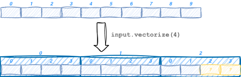
rank = input.shape().size();              // Number of dimensions: 2
int vCount = input.dim(0);                // Number of vectors: 3
vCount= input.dim(Vectorized::Vectors);   // Same as above
int vSize = input.dim(1);                 // Number of items in each vector: 4
vSize = input.dim(Vectorized::Elements);  // Same as above
slice.iram.load(input[0]);                // Load the first vector
slice.iram.load(input[0][2]);             // Load the third item of the first vector
Choosing the right vector size is important for optimal performance. Ideally should be as large as possible without going beyond the capablities of the ALU and Act units. The ALU supports larger vector sizes than the Act, furtermore the vector size for input data can be different from that for weights data. Why this difference between ALU and Act? Many of the most common kernels are accumulating kernels, that is the ALU must process multiple input data before the generated partials can be send to the Act for processing (see for example the reduce kernel in the tutorial). This means that a large vector size in Act is not needed, because while the ALU is processing the input values to generate the next partial, the Act has all the time to process the previous partials in smaller chunks.
The rule of thumb for choosing the vector size is summarized here below.
Important
For non accumulating kernels get input vector size from Act
width()method.For accumulating kernels get input vector size from Alu
iWidth()method.Weight vector size is always available via the Alu
wWidth()method.
Note that the input vector size is also affected by the data type of the weights, so if weights
are used iWidth() must be called with both types specified.
When using an input vector size greater than Act vector size, the partials generated by the Alu
cannot be processed in one go by the Act .
The PData structure returned by the Alu instruction is already divided in sub-tensors of the right
size to be processed by the Act, it’s enough to iterate on the PData::Vectors dimension
(see the Matrix Reduce example in the tutorial).
Important
Vectorizing output tensors is not necessary and deprecated since the last vector may go beyond the
end of the tensor. This can make the store() or append() instruction write outside the
tensor boundary (this will normally generate an assertion).
Writing output results
The Slice class provides two methods for writing results to the output tensor:
store(output[...], res)append(output[...], res)
where […] represents any number of indexed dimensions.
Each of the two methods has advantages and limitations.
store(output[...], res) will write the res tensor into the [sub]tensor specified in the first parameter.
The constraint is that the number of elements in the two tensors must match. The advantage is
that any part of the output tensor can be written in any order by indexing the desired part of the tensor.
append(output[...], res) will instead append res to the results already written to the
output[…] [sub]tensor. It’s not possible to write the content of this subtensor in a different order,
but it’s still possible to generate multiple subtensors in parallel.
There is no requirement for res to match the size of the subtensor being written.
Furthermore it never overflows the size of the output (sub)tensor it is writing, if some data would
go past the end of the specified output (sub)tensor it is simply discarded.
For example if we try to append two 16-bytes results to a tensor of size 20, the first append will write the
entire 16 bytes, while the second append will just write the initial 4 bytes and discard the remaining 12.
This makes append() the ideal choice in most cases since it allows to handle in a natural way
output tensors of any size without requiring any additional padding.
It may not be clear which dimensions have to be specified for the output tensor used in append().
Can’t we just call append(output, res) without specifying any index?
The rule is that if the computation of a given dimension may go beyond the end of the
dimension itself, then we should append to that dimension, so that the append method will avoid
the overflow. For example if we are processing a 2D tensor one row at a time, and we process
each row 64 values at a time, then we can call append(output[rowIndex], res) to ensure we will
not write beyond the end of each row even if it is not a multiple of 64.