The prefetch list scheduler

How PrefetchInputsPass reorders a function’s NSS stream so that DMA transfers overlap slice compute. Everything here follows compiler/torq/Codegen/PrefetchInputsPass.cpp: StreamGraph, simulateOrder, listSchedule and PrefetchInputsPass::runOnOperation.

• 1. The problem

• 2. The hardware model

• 3. Where the pass runs and what it sees

• 4. Step 1: the dependency graph (StreamGraph)

• 5. Step 2: the scheduling loop (listSchedule)

• 6. Worked example 1: overlap and both slices

• 7. Worked example 2: the LRAM limits

• 8. Step 3: choosing a schedule (runOnOperation)

• 9. The tile budgets

• 10. Limits and known gaps

• 11. Flags

---

1. The problem

After lowering, a function is one long in-order NSS control stream:

load  w1          ; DMA XRAM -> LRAM, blocks the stream
start P1          ; slice runs P1, the stream goes on
wait  P1          ; blocks until P1 is done
load  w2
start P2
wait  P2
...
store out         ; DMA LRAM -> XRAM, blocks the stream

Written like this, the DMA engine and the slices take turns: while P1 computes, nothing is loading w2, and while w2 loads, both slices are idle. The list scheduler rewrites the order of these operations (and which slice runs each program) so that loads, stores and compute overlap, without changing what is computed and without exceeding LRAM.

2. The hardware model

              NSS stream (in order, one op at a time)
                 |            |             |
                 v            v             v
          +-------------+  +---------+  +---------+
          |  DMA engine |  | slice 0 |  | slice 1 |
          | (loads AND  |  +---------+  +---------+
          |  stores)    |
          +-------------+
                 \            |             /
                  +------- LRAM (512 KB) --+

op	what it does to the stream	time model in the scheduler
torq_hl.load	blocks until the transfer is done	t = max(t, dmaFree) + dur; dmaFree = t
torq_hl.store	blocks until the transfer is done	same as a load: one DMA engine for both
start_program	asynchronous, the stream goes on	slice busy until t + compute; t += 1
wait_program	blocks until that program ends	t = max(t, sliceEnd)

The durations come from the IR. Load cycles come from dmaCyclesForLoad. Store cycles come from the torq-async-duration-cycles attribute, and compute cycles from the slice_profiling annotations that AnnotateDmaAndSliceCyclesPass adds just before this pass.

The makespan is max(t, dmaFree) after the last op. simulateOrder computes it for any order with exactly these rules, and that is how the input order is priced.

3. Where the pass runs and what it sees

The pass runs only with --torq-prefetch-algorithm=stream-schedule. The default, auto, is constant-loads (torq-prefetch-constant-loads) on every chip, so a compile without the flag does not change. Only one prefetch algorithm runs in a compile.

TileAndFuse -> ... -> bufferization -> slice programs outlined
  -> ConvertSliceProgramToTorqHw
  -> AnnotateDmaAndSliceCycles        (durations)
  -> PrefetchInputs   <== here (--torq-prefetch-algorithm=stream-schedule)
  -> AddDeallocation -> RecoverLramResidency -> AssignLramAddresses

It runs before LRAM addresses are assigned. The buffers are still memref.allocs, so the scheduler is free to reorder. It has to predict whether the allocator can place the new order, and it checks that by running the real allocator on a clone (section 8).

4. Step 1: the dependency graph (StreamGraph)

Every op in the block becomes a node of one of six kinds:

kind	ops	scheduled?
Pure	memref.alloc, constants, views, invocations, program bodies	no: emitted just before the first action that needs it
Load	torq_hl.load	yes, on the DMA engine
Store	torq_hl.store	yes, on the DMA engine
Start	start_program of a slice invocation	yes, on a slice
Wait	its matching wait_program	yes
Barrier	anything else (host/CSS calls, a start without a wait, …)	yes, keeps its place

Edges (A -> B means A must come first):

1. SSA: B uses a value A defines, including values used inside B’s regions.

2. Program: start P -> wait P.

3. Barriers: everything since the previous barrier goes before a barrier, and a barrier goes before everything after it.

4. Memory: two accesses to overlapping byte ranges of the same buffer, at least one of them a write, keep their input order. This covers read-after-write, write-after-read and write-after-write, in LRAM and in XRAM. A program holds its buffers until its wait, so an edge out of a program starts at its wait.

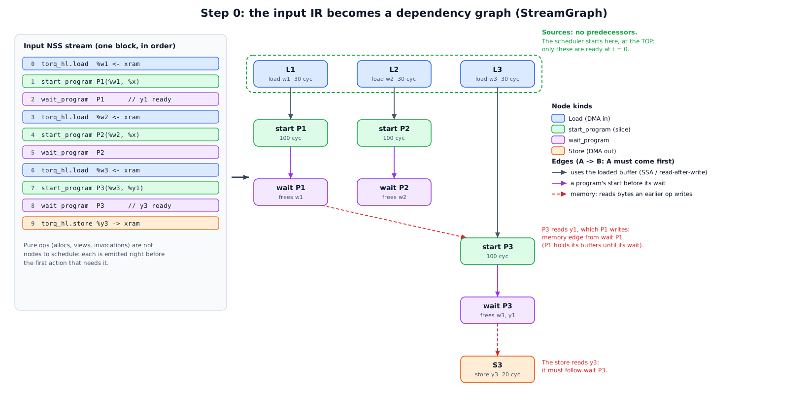
   load w1 ---> start P1 ---> wait P1 ---+
                                          |  (P3 reads P1's output o1)
   load w3 -------------------------------+--> start P3 ---> wait P3 ---> store out
   load w2 ---> start P2 ---> wait P2

The graph also records, for the LRAM model:

• allocBytes_: the size of every LRAM buffer. It is born when its alloc is emitted, which happens just before its first user.

• userAllocs_ / allocUserCount_: who uses each buffer. It dies after its last user, and for a program that is the program’s wait.

• startBuffers_: the buffers each program touches. They are used to mark a load as “urgent” (section 5).

• firstConsumer_: the first program that reads a load’s buffer. It is used for the “reserve” (section 5).

5. Step 2: the scheduling loop (listSchedule)

A classic list scheduler: keep a set of ready actions (all predecessors already emitted), and at each step pick one ready action and emit it. The policy plays out the hardware of section 2 on a simulated clock.

State

t	current position of the in-order stream, in cycles
dmaFree	when the DMA engine is free
sliceProg[s], sliceEnd[s]	program running on slice s (or none), and when it ends
live	LRAM bytes currently alive
space	an LramAddressSpace of cap bytes: real offsets, two-ended first fit
ready sets	readyStarts, readyDmas (loads and stores), readyWaits, readyBarriers, each oldest first

LramAddressSpace mirrors the real allocator’s policy. Buffers under 8 KB go bottom-up and larger ones top-down, so small buffers do not fragment the space the large ones need. A buffer “fits” only if every buffer the action creates gets a real contiguous range, not just if the byte total is under cap.

One step: the decision order

flowchart TD
    A[step] --> B{barrier ready?}
    B -- yes --> B1[emit barrier]
    B -- no --> C{a slice free?}
    C -- yes --> C1{oldest ready start\nwhose buffers fit?}
    C1 -- found --> C2[start it on the first free slice\nsliceEnd = t + compute; t += 1]
    C1 -- none, and no slice running --> C3[force the oldest ready start]
    C1 -- none, a slice running --> D
    C -- no --> D{oldest ready load/store\nthat fits?}
    D -- found, and it can start\nbefore the first running\nprogram ends --> D1[emit it\nt = max t,dmaFree + dur]
    D -- otherwise --> E{a program running?}
    E -- yes --> E1[emit the wait of the slice\nthat ends first\nt = max t, sliceEnd; slice free]
    E -- no --> F[emit the oldest ready load/store,\nor the oldest ready action]

In words:

1. Barrier ready: emit it at once.

2. A slice is free: take the oldest ready start (looking at no more than 32) whose new buffers all get an address under cap. Put it on the first free slice. If none fits and no slice is busy, start the oldest one anyway, so the schedule cannot deadlock.

3. The DMA engine: take the oldest ready load or store (no more than 32 again) that fits:

   • a store always fits, because it frees memory;

   • a load for one of the next urgentStarts (4) programs may use all of cap;

   • any other load (a prefetch for a program further ahead) may only fill LRAM up to prefetchCap (40% of cap);

   • every load also leaves a reserve: room for the largest program that starts before the load’s consumer. The loaded buffer stays alive across those programs, so they must still fit next to it.

   Emit the transfer only if it can start before the first running program ends (max(t, dmaFree) <= earliestEnd). Otherwise the stream would sit in a transfer while a slice goes idle.

4. Otherwise wait: emit the wait of the slice that ends first. Its buffers are released, and the slice is free.

5. Nothing applies: emit the oldest ready load or store, or the oldest ready action, so it always makes progress.

Emitting an action also emits, just before it, every pure op it needs that is not out yet: its allocs, views and invocation. That is where its buffers are born (append). Emitting the last user of a buffer releases it from space.

The result is the new op order, the slice of every program (sliceOfStart, which becomes the invocation’s executor_id), the predicted makespan and the peak live bytes.

6. Worked example 1: overlap and both slices

Three programs, plenty of LRAM:

	needs	compute
P1	weights w1 (load L1, 30 cycles)	100
P2	weights w2 (load L2, 30 cycles), independent of P1	100
P3	weights w3 (load L3, 30 cycles) and P1’s output	100
S3	store of P3’s output, 20 cycles

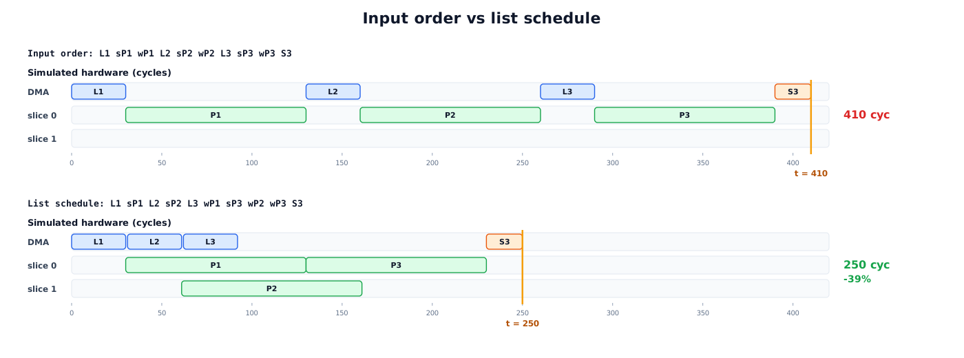
Input order, priced by simulateOrder:

L1 start P1 wait P1 L2 start P2 wait P2 L3 start P3 wait P3 S3

t:   0    30        130 160        260  290        390   410
DMA  [L1]           [L2]           [L3]                [S3]
s0       [----P1----]  [----P2----]   [----P3----]
s1       (idle the whole time)
makespan 410

listSchedule, step by step. At the start L1, L2 and L3 are ready, and no start is ready.

step	t before	slices	rule	emits	t after
1	0	s0 free, s1 free	2: no ready start. 3: L1 is urgent and fits, no program running	L1	30
2	30	both free	2: P1 ready, fits	start P1 -> s0 (ends 130)	31
3	31	s1 free	2: P2 not ready. 3: L2 starts at 31 <= 130	L2	61
4	61	s1 free	2: P2 ready	start P2 -> s1 (ends 161)	62
5	62	none free	3: L3 starts at 62 <= 130	L3	92
6	92	none free	3: nothing ready (S3 needs P3). 4: s0 ends first	wait P1	130
7	130	s0 free	2: P3 ready (L3 done, P1 done)	start P3 -> s0 (ends 230)	131
8	131	none free	4: s1 ends first (161)	wait P2	161
9	161	s1 free	2: nothing ready. 4: s0 running	wait P3	230
10	230	both free	3: S3 ready, nothing running	S3	250

new order: L1 start P1 L2 start P2 L3 wait P1 start P3 wait P2 wait P3 S3

t:   0    30 61 92     130            230   250
DMA  [L1][L2][L3]                      [S3]
s0       [-----P1-----][-----P3-----]
s1           [-----P2-----]
makespan 250   (-39%)

Two things happened. L2 and L3 load while P1 computes (rule 3), and P2 runs on slice 1 next to P1 (rule 2, first free slice). The memory edge wait P1 -> start P3 still holds, so P3 reads P1’s finished output.

The same example, picture by picture

Each step figure has five parts:

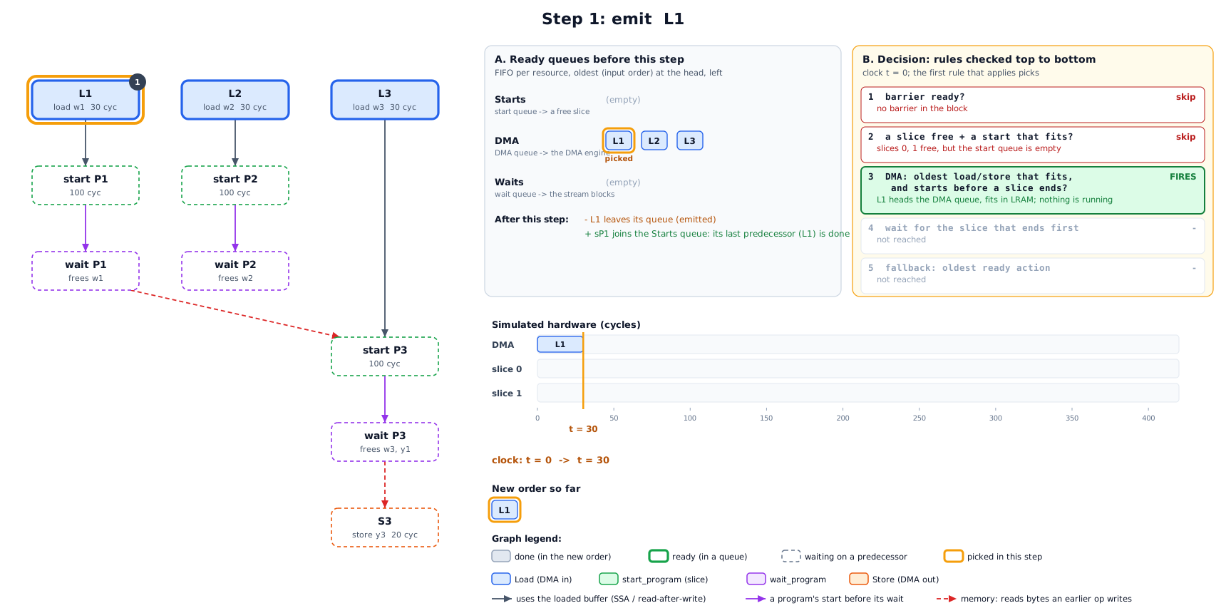
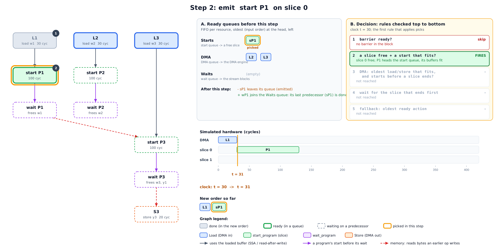
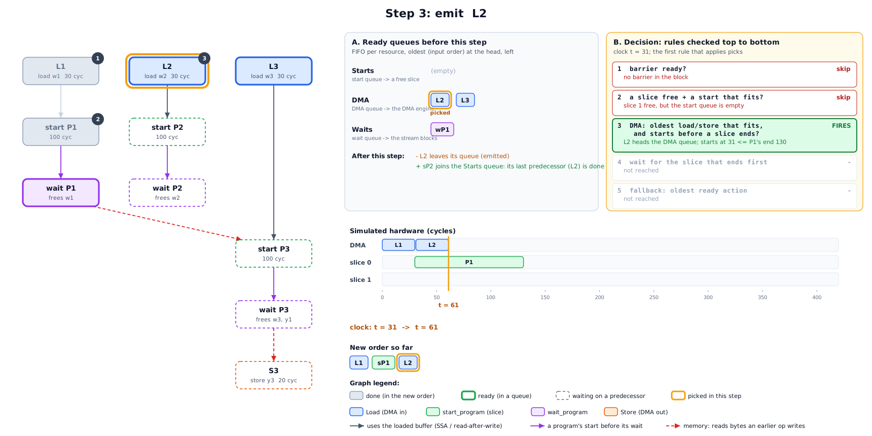
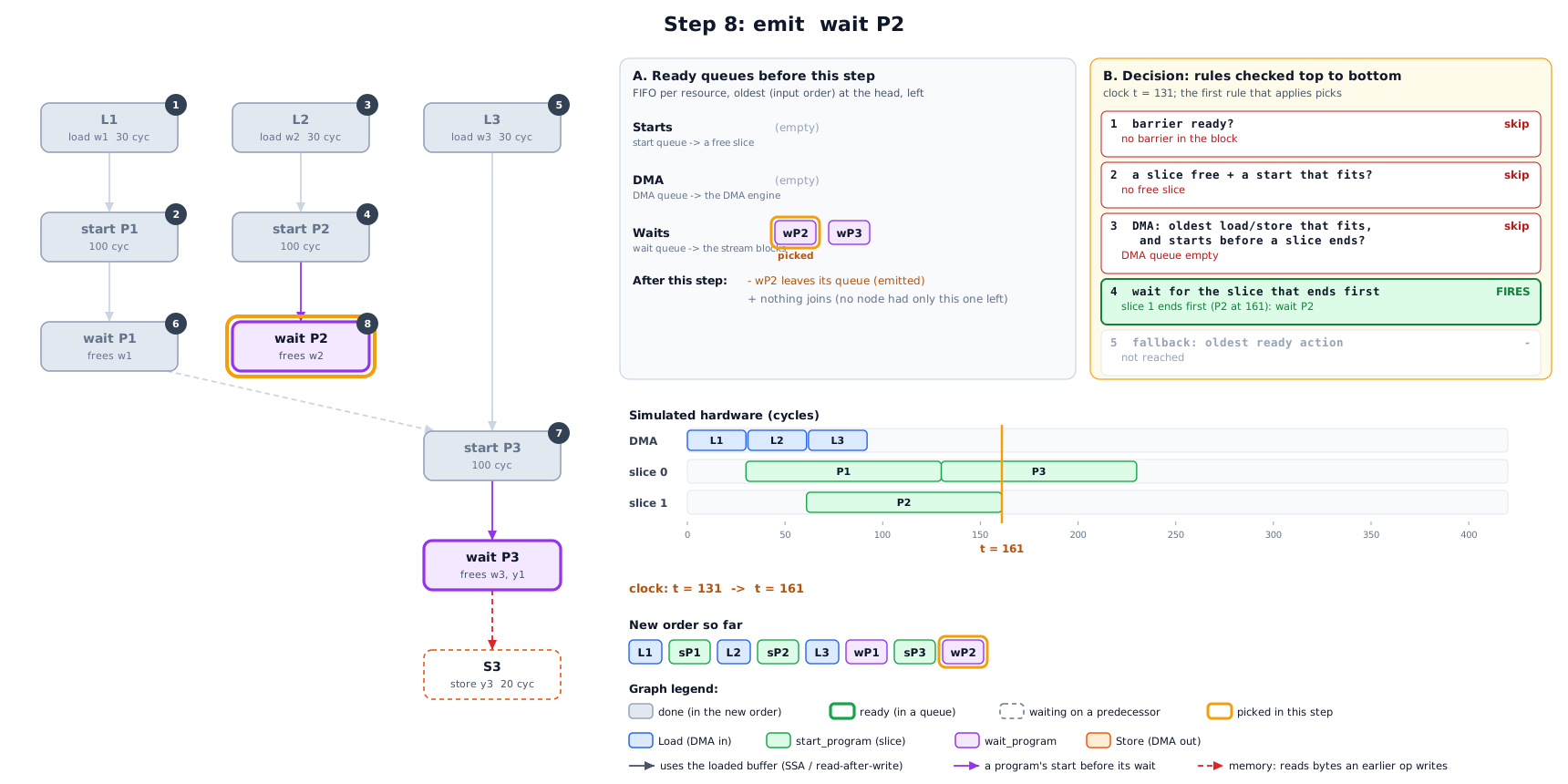
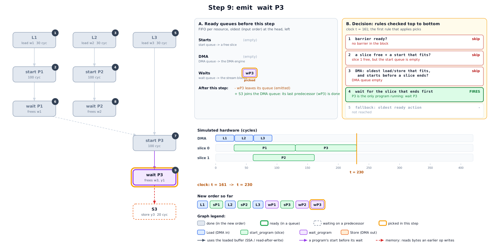
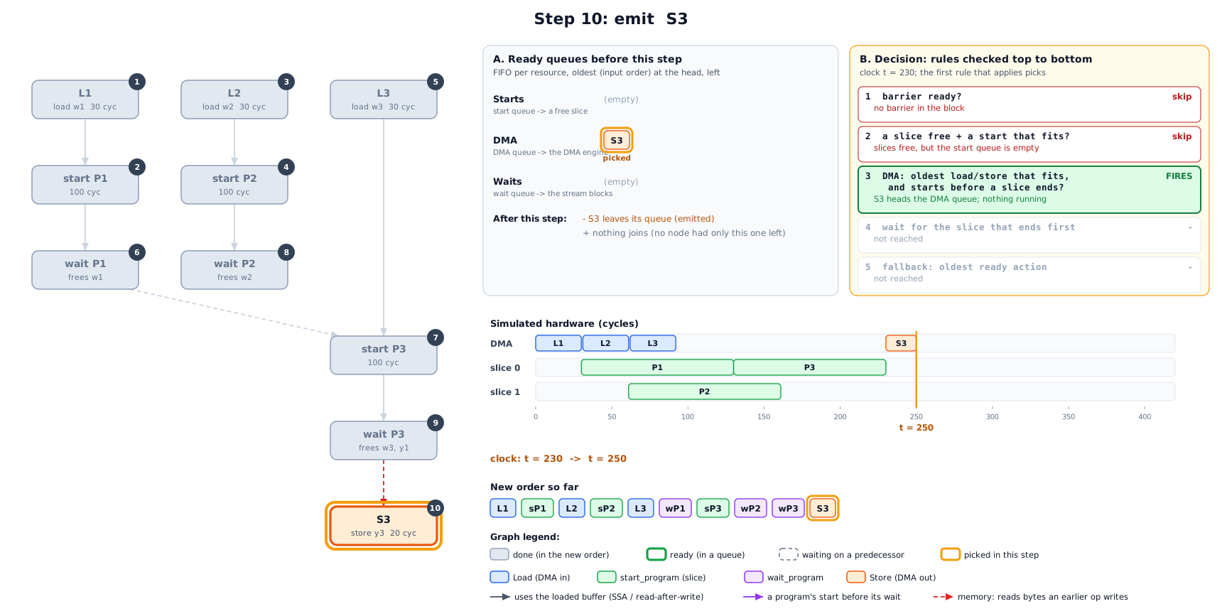
• The graph (left): grey nodes are already emitted, numbered by the step that emitted them. Thick outlines are ready, dashed nodes are still waiting on a predecessor, and the orange box is the node picked in this step.

• A. Ready queues: every ready node sits in the FIFO queue of the resource that runs it: starts go to a slice, loads and stores to the DMA engine, and waits block the stream. Each queue is oldest first, by input order. Under the queues: which node leaves (the one emitted), and which nodes join because the emitted node was their last missing predecessor.

• B. Decision: the five rules of section 5, checked top to bottom. The first rule that applies picks the node from the head of its queue. Every rule above it is marked skip with the reason, and every rule below is not reached.

• Simulated hardware: the DMA engine and both slices, up to the current clock (orange line).

• The new order built so far.

Where does it start? At the top of the graph. The scheduler walks forward in time, not backwards from the result. At t = 0 the only ready nodes are the sources, the nodes with no predecessors: here the three loads. A node becomes ready the moment its last predecessor is emitted. Among ready nodes, the rules of section 5 decide, and ties go to the oldest one in the input order.

Step 0: the IR becomes a graph. Each NSS op is a node. Its kind decides which resource runs it (DMA engine or slice). Edges are the orderings that must be kept.

Step 1: no program is ready yet, so the DMA engine takes the oldest ready load.

Step 2: P1’s input is in, so P1 starts on the first free slice, slice 0. start does not block, and the stream moves on at t + 1.

Step 3: P2 is not ready, but L2 can start before P1 ends. This is the overlap: w2 loads while P1 computes.

Step 4: P2 is ready and slice 1 is free, so both slices now compute.

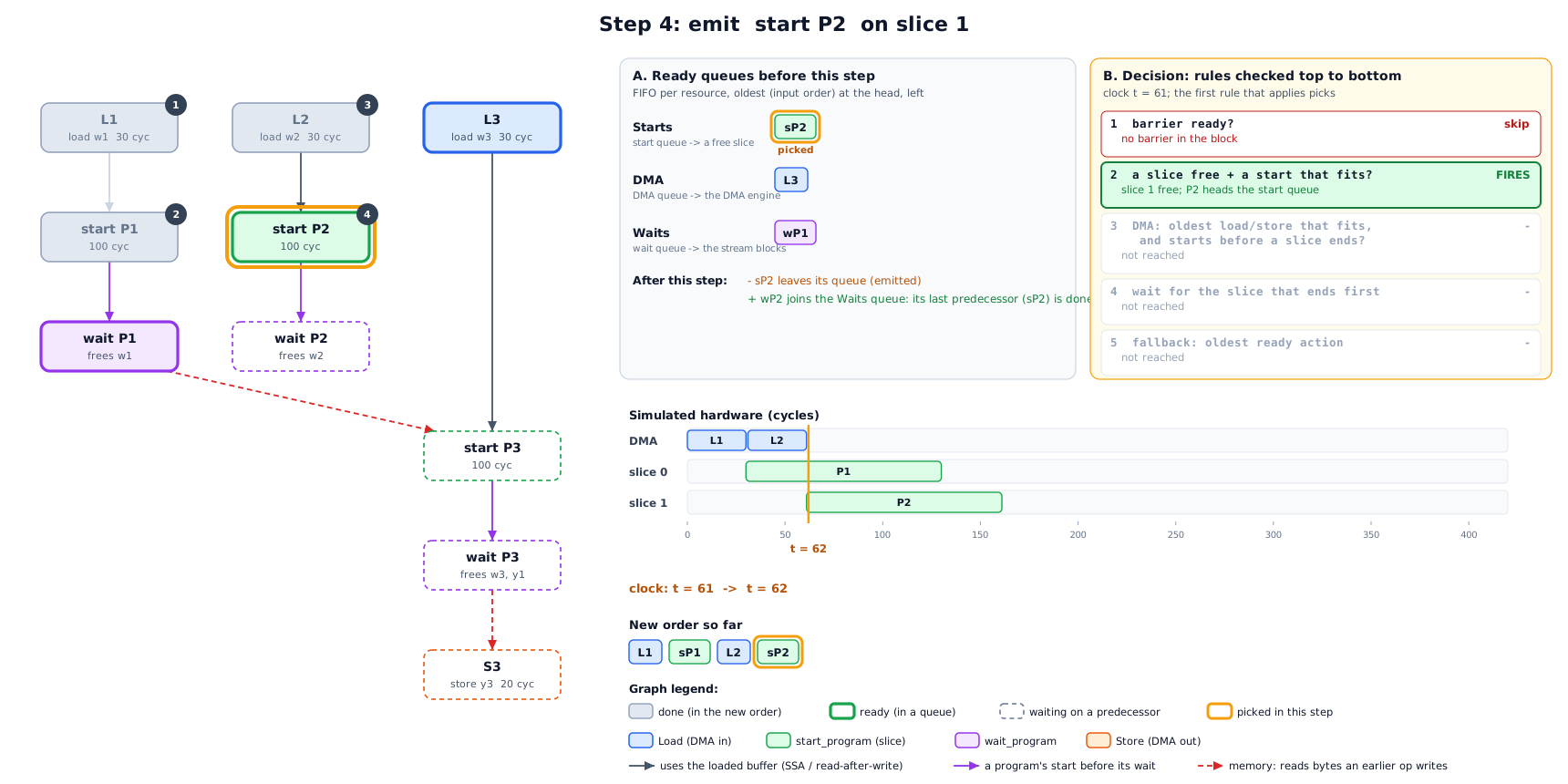
Step 5: no slice is free, and L3 still starts before the first program ends: w3 is prefetched for P3.

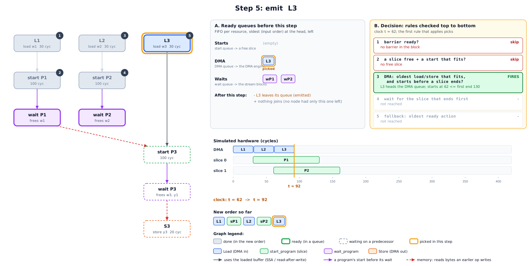
Step 6: nothing useful is left for the DMA engine, so the stream waits for the slice that finishes first (P1). That frees slice 0 and P1’s buffers.

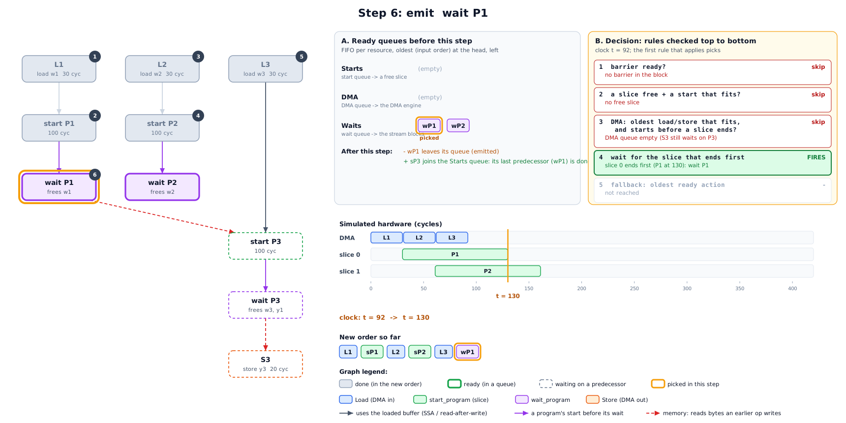
Step 7: P3 is ready only now: its weights are loaded and P1’s output is final. It goes on slice 0.

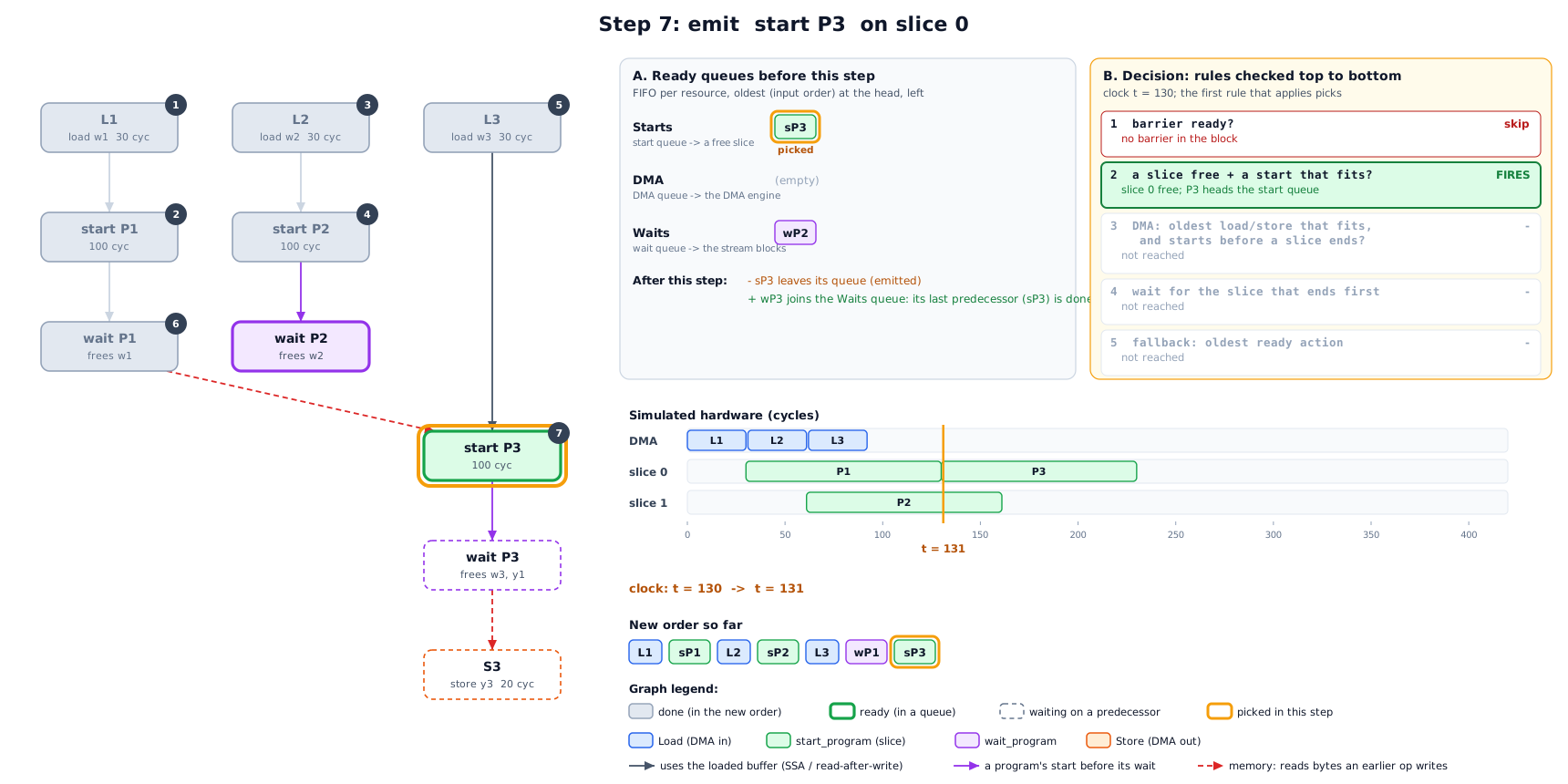
Steps 8 to 10: wait for P2, then P3, then store P3’s output.

Result:

7. Worked example 2: the LRAM limits

The same rules decide how far ahead a load may go. Take cap = 100 KB, so prefetchCap = 40 KB. Use urgentStarts = 1 to keep it short (the real default is 4). Five programs follow each other. Each needs one 30 KB weight buffer and writes one 30 KB output, and P1 is running with 30 KB live.

load	for	urgent?	limit	live + load + reserve	decision
L2	P2 (next)	yes	100 KB	30 + 30 + 0 = 60	emit
L3	P3	no	40 KB	60 + 30 + 30 = 120 > 40	wait

The reserve for L3 is P2’s 30 KB output. P2 starts before L3’s consumer P3, and that buffer is born when P2 starts. P2’s weights do not count: L2 already brought them in.

L3 is held back. It is a prefetch for a program two steps away, and LRAM is already over the prefetch cap. Once wait P1 frees P1’s weights and P2 starts, P3 becomes the next program, so L3 is urgent and may use the full cap.

Without these limits the scheduler would greedily load weights for programs far ahead and fill LRAM. The near programs would then not fit, and the allocator would have to insert swaps (spill and reload DMA), which costs more than the overlap gains.

8. Step 3: choosing a schedule (runOnOperation)

listSchedule only predicts. The pass then asks the real allocator (on a clone) what the order costs:

flowchart TD
    G[build StreamGraph\nprice the input order: inputPredicted] --> P0
    subgraph P0 [pass 0: no swaps allowed]
      direction TB
      a1[for cap in 100%, 85%, 70% of usable LRAM] --> a2[listSchedule]
      a2 --> a3{predicted < inputPredicted?}
      a3 -- no --> a1
      a3 -- yes --> a4{real allocator places it\nwith no swaps?\norderPlacesInLram}
      a4 -- no --> a1
    end
    a4 -- yes --> DONE[commit order + slice ids]
    P0 -- no cap placed --> P1
    subgraph P1 [pass 1: swaps allowed]
      direction TB
      b1[same three caps] --> b2[listSchedule]
      b2 --> b3[real allocator WITH swaps\nsimulateStream -> makespan]
      b3 --> b4[keep the fastest: bestList]
    end
    P1 --> LO{bestList faster than the input order,\nalso priced after allocation?}
    LO -- yes --> K[commit bestList]
    LO -- no --> IN[keep the input order]

• Pass 0 wants a schedule the allocator places without a single swap. A smaller cap leaves the allocator slack the model cannot see: alignment, fragmentation, NSS program slots. On most functions the first cap places, and the pass stops there.

• Pass 1 runs only when no cap placed. It asks whether a schedule still beats the input order when the allocator’s swaps are included. Each candidate is priced after allocation, its swaps included, and the fastest is kept. This occurs mostly when the input order itself needs more LRAM than exists, so the allocator swaps whatever the order. A schedule with a few swaps can also beat an input order that places without swaps, when its overlap gains more than the swaps cost.

• A schedule must beat the input order. The prediction cannot see swaps, so it is the bar only when the input order places without them. When the input order needs swaps, the bar is its real cost after allocation.

• If no schedule beats the input order after allocation, the input order is kept, so the pass never makes a block slower by its own measure.

Every attempt runs the real allocator on a clone, so a block pays at most 3 allocator runs in pass 0, plus 3 more in pass 1.

9. The tile budgets

The scheduler can load a weight early only when LRAM has free space for it. TileAndFuse normally sizes every tile against the whole LRAM, so a tile that fills LRAM leaves no space for the next load. With stream-schedule, TileAndFuse sizes some tiles against a smaller part of LRAM, the tile budget. Only the tile-fit probe sees the smaller budget. The real pipeline still allocates into the whole LRAM, so the free space is there for the scheduler.

TileAndFuse first looks at the whole function:

function	budgets
constants fit in LRAM	the whole LRAM for every loop, as without the flag. The weights load one time and stay, so there is nothing to stream.
constants > LRAM	every loop gets --torq-prefetch-tile-budget-percent (default 50), except the matmul loops, which get --torq-prefetch-matmul-tile-budget-percent (default 40). FoldConvert sizes against --torq-prefetch-tile-budget-percent, because the probe and the real pipeline must keep the same data in LRAM.

• A matmul loop is a tile loop rooted at a contraction (a matmul). The smaller tile costs it no halo, and the next weight tile loads while the current tile computes. A 52 MB int4 LM head (one matmul) goes from 25.9 ms to 13.7 ms on the board.

• The matmul tile must not split the rows. The rows are the parallel dimensions the weight does not index. If the smaller budget splits them, each row tile loads the whole weight again (matmul 1x128x768x3072 bf16: 2 x 64 rows load a 4.7 MB weight two times, +91%). Then the loop fits against the whole LRAM.

• All the loops of the function. The free LRAM lets the next layer’s weights load while the current layer computes. gemma3 hybrid: 61.0 ms with the smaller budget on the matmul loops only, 54.9 ms with it on all the loops.

• Convolution models are not tuned yet. A convolution pays for a smaller tile with halo reloads and recompute, so a convolution model can be slower with stream-schedule. Do not use it for convolution models yet.

10. Limits and known gaps

• No swaps in the model. The scheduler assumes everything it schedules stays in LRAM. When the input order itself is over LRAM, pass 0 cannot place, and on some models the schedule is predicted slower than the input order and is dropped. This occurs on convolution models whose tiles fill LRAM (section 9).

• FIFO policy. “Oldest ready first” is simple and keeps the order close to the input, but it is not critical-path aware. A long chain is not started earlier than its position says.

• First free slice. No load balancing: a program goes to whichever slice is free first. Splitting one op across both slices is LinalgSlicing’s job, earlier in the pipeline.

• 32 candidates per step. This bounds compile time on large functions, where thousands of weight loads are ready from the start.

• Predicted vs real. The DMA and compute cycles are estimates (the same ones the compile-time profile uses), so a predicted gain is checked against the real allocator, never trusted on its own.

11. Flags

All flags apply only with --torq-prefetch-algorithm=stream-schedule, except the algorithm flag itself.

flag	default	meaning
--torq-prefetch-algorithm	auto	stream-schedule (this pass and the tile budgets of section 9), constant-loads (torq-prefetch-constant-loads), or none. auto is constant-loads
--torq-prefetch-tile-budget-percent	50	percent of LRAM the tile-fit probe may use in a function whose constants do not fit in LRAM. FoldConvert uses it too (section 9)
--torq-prefetch-matmul-tile-budget-percent	40	percent of LRAM for a matmul tile loop in a function whose constants do not fit in LRAM (section 9)
--torq-list-cap-percent	100	first cap, in % of usable LRAM (then x0.85 and x0.70)
--torq-list-prefetch-percent	40	prefetchCap, in % of cap, for loads of far programs
--torq-list-urgent-starts	4	how many upcoming programs count as near